In order to determine the operating pressure and flow of the entire system, an Excel calculator was built to determine the pressure drops of each individual tubing run, fitting, and hydraulic device in the loop.

By calculating these pressure drops, the resulting pressure versus flow (or “PQ”) curve was overlayed onto the Davies Craig EBP40 24V PQ curve to determine the point of intersection. The point of intersection tells us the pressure the pump will provide to overcome the pressure drop of the entire system. As a result of determining this theoretical point, the flowrate of the loop is also quantified.

This article explains how the hydraulic losses were calculated, and the final pressure and flow of the loop.

---

Major and Minor Losses

The hydraulic performance of different devices can be quantified using 3 different methods: analytical calculations, CFD, or empirical testing. The table below shows how each device was quantified.

Hydraulic Device	Method for Pressure Drop Calculation
Straight tubing runs	Darcy-Weisbach equation
90deg tubing runs	Minor loss coefficients
Fittings	Minor loss coefficients
Valves	Minor loss coefficients
Motor jackets	CFD
Cold plates	CFD
Radiators	EV5 empirical data

Table 1 Methods for pressure drop calculations

Major Losses

Major losses were calculated using the Darcy-Weisbach equation as shown below.

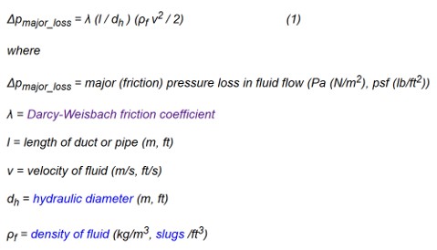
Fig. 1 Darcy-Weisbach equation

In order to use the above equation, the friction coefficient (lambda) is needed. It is obtained using the Colebrook equation, shown below.

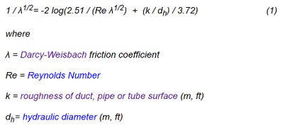
Fig. 2 Colebrook equation. This is simply an analytical implementation of a Moody diagram, therefore it is preffered to use this equation for precise design

Finally, in order to use the Colebrook equation, you need the absolute roughness coefficient (k), which can be obtained using the chart below.

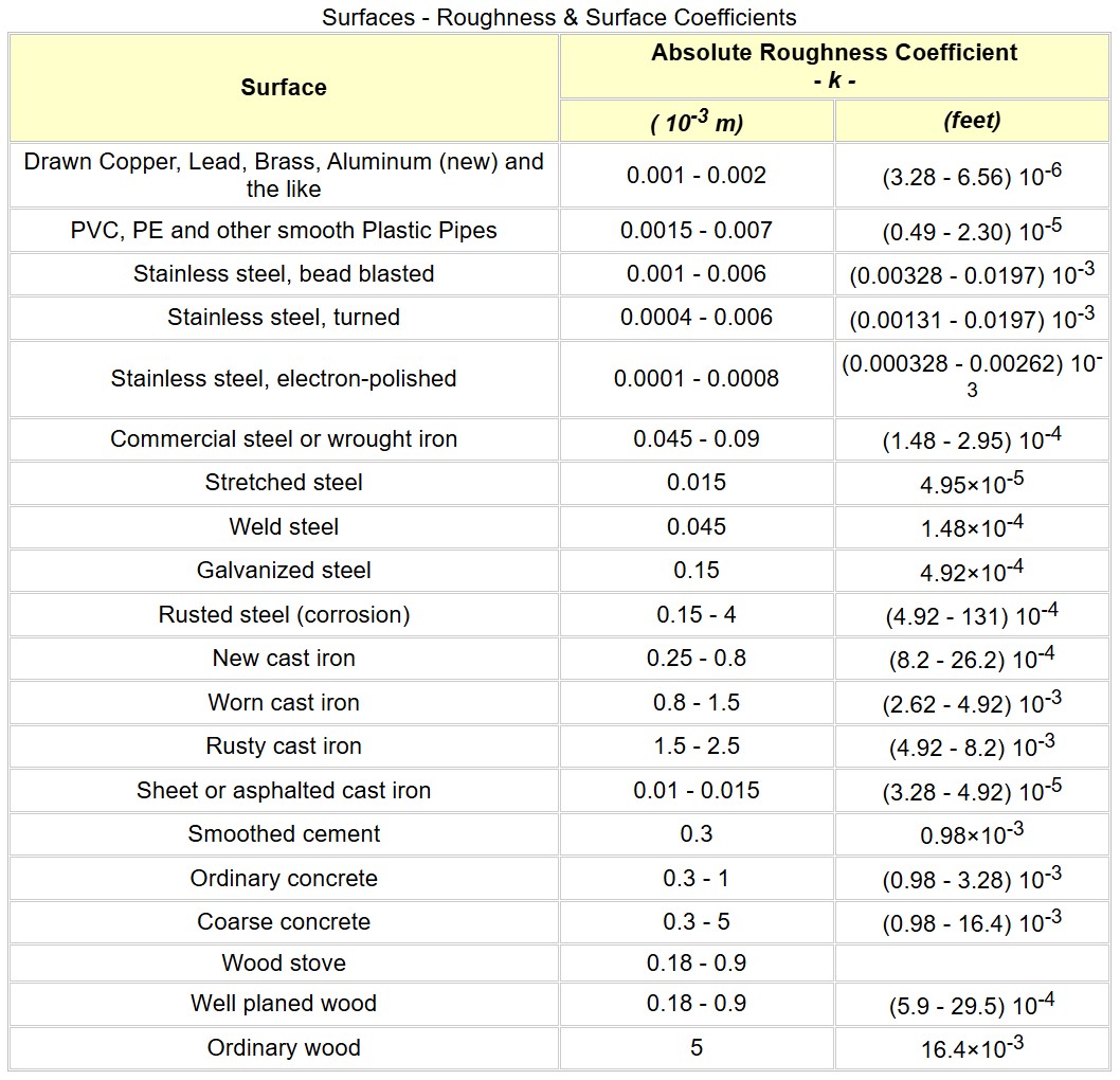
Fig. 3 Absolute roughness coefficient chart

Minor Losses

Minor losses were calculated using minor loss coefficients, using the equation below.

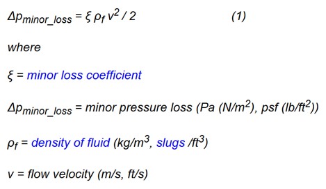
Fig. 4 Minor loss coefficients equation

In order to use the above equation, the minor loss coefficient is needed. It is obtained using the chart below.

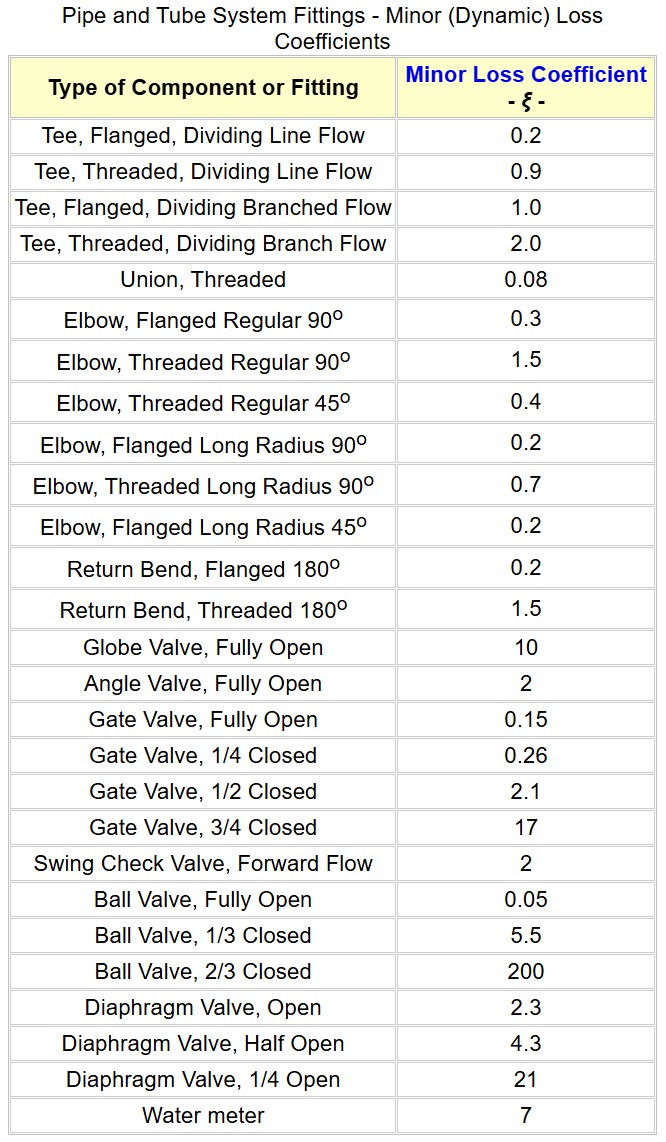
Fig. 5 Minor loss coefficients

If the fitting being evaluated is a reducer, a different equation is used to calculate the minor loss coefficient. It is shown below.

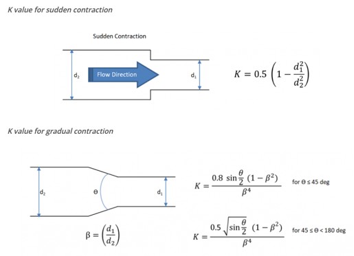
Fig. 6 Minor loss coefficient equations for reducers

All of the formulas explained above were integrated into an Excel calculator to automatically calculate the pressure drop of a given tubing run, fitting, or valve. The workbook takes CAD measurements and fluid properties (flow rate, density, and viscosity) as the input, and outputs the pressure loss for the given device.

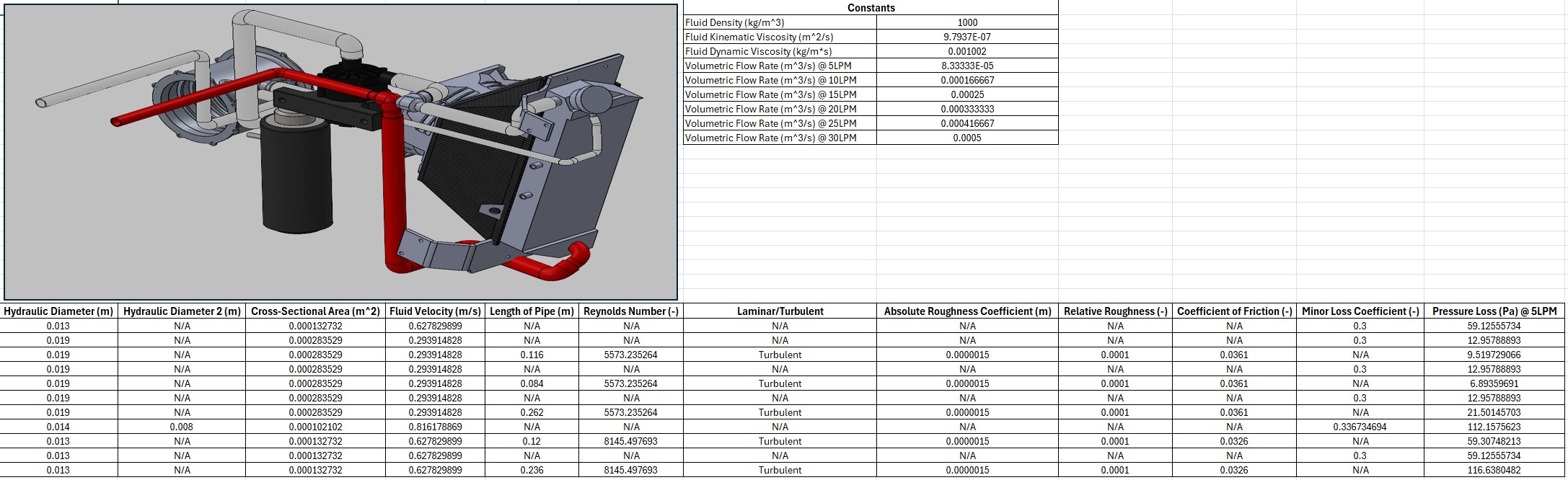
Fig. 7 Excel calculating the pressure drop of the "red" coloured section in the CAD screenshot. The table shown is specifically calculating for pressure drop at 5LPM. All flowrates are calculated to draw the final PQ curve

---

System PQ Curve

By using the Excel calculator explained earlier in this article, the operating point of the MACFE 2025 cooling loop is shown in the intersection of the PQ curves below.

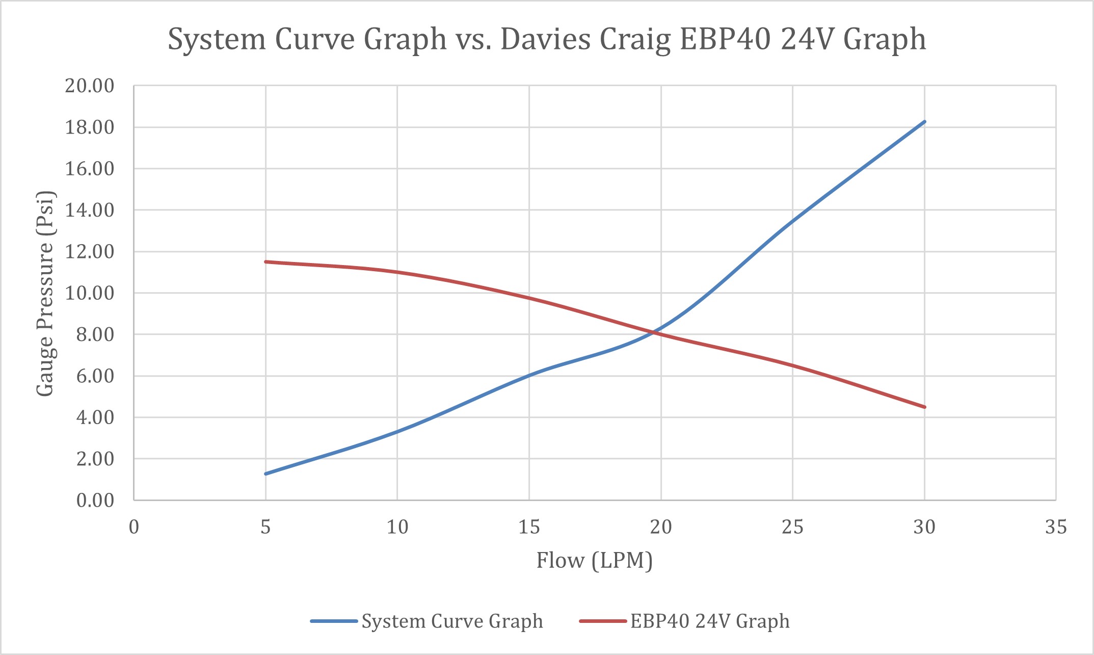
Fig. 8 EV6 cooling system operating point

---

System Architecture

An overall system architecture flowchart was made to make the hydraulic flow path easy to understand. This PDF document was then given to the Chassis subteam for tubing routing and implementation. Note that the fittings in the document seen below may have changed based on what was implemented on the actual car, due to packaging and budget reasons.

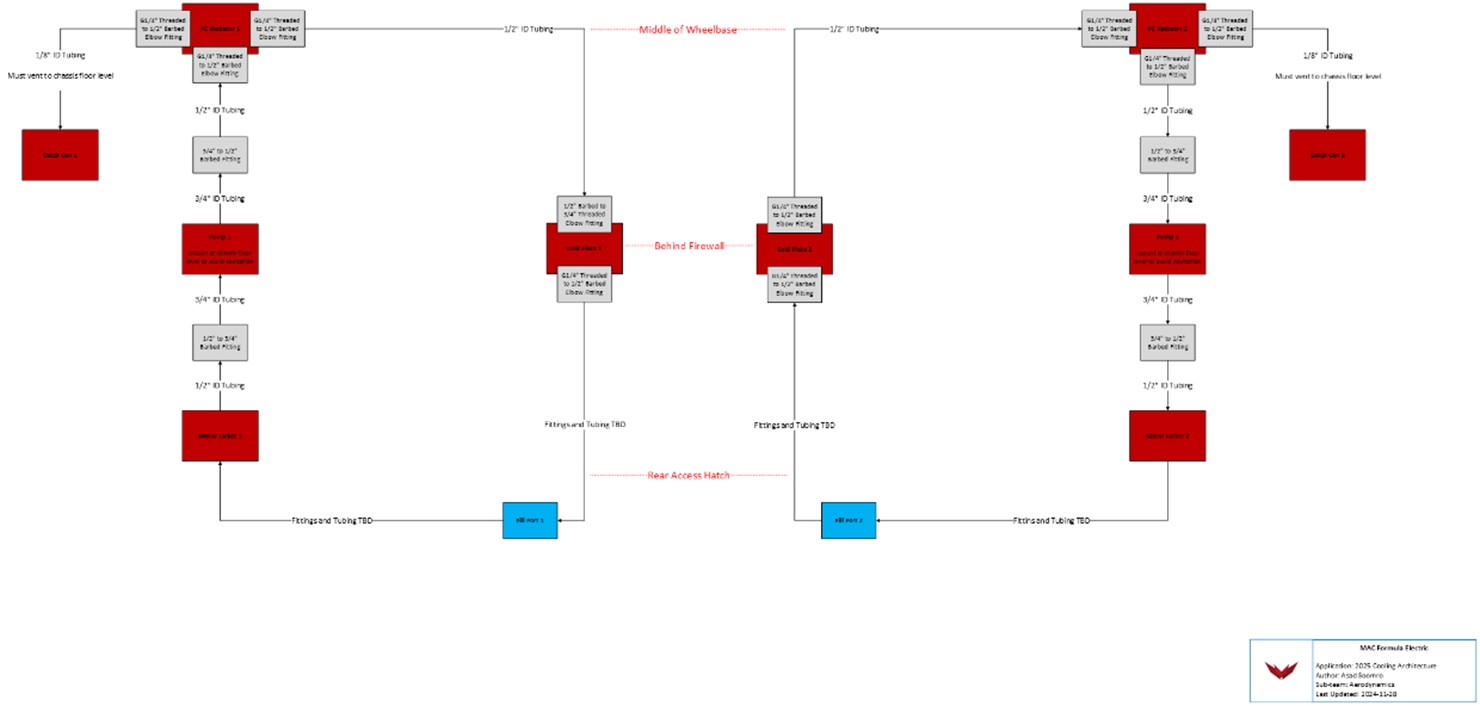
Fig. 9 EV6 cooling architecture