In order to quantify the operating point of the MACFE 2025 cooling loop, the pressure drop across all circuit components needs to be determined. For custom designed components such as the motor jackets and inverter cold plates, it would need to either be determined experimentally or through CFD analysis. Due to time and budget constraints, we proceeded with the latter.

The results of this article were then integrated into a major and minor losses calculator to find the operating point. This will be documented in a post directly following this one.

---

Motor Jackets

Y+ Calculation

Firstly, the target volume flow rate of 10LPM was converted to velocity using the hydraulic diameter of the motor jacket inlet:

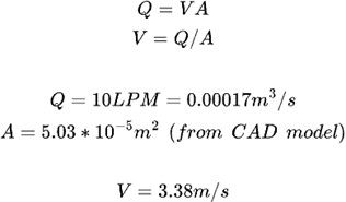
Fig. 1 Velocity calculation

Using the velocity, we are now able to calculate the required wall spacing for our desired y+ value. The specific calculator used is linked here.

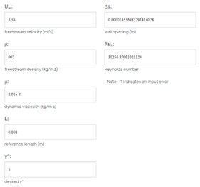
Fig. 2 Wall spacing calculation

The freestream density and dynamic viscosity were the properties of water taken at SATP. The reference length is the internal diameter of the inlet tube of the motor jacket. The wall spacing was taken and used in the boundary layers of the mesh.

It should be noted that in the future, the y+ value should be calculated using the maximum analyzed volume flow rate. In our case, the wall spacing was calculated at 10LPM as that was the initial targeted flow rate for the system. However, it is better practice to calculate it at the maximum possible flow rate, which in our case is 37LPM since the pump’s PQ curve is tested to 37LPM, as shown below:

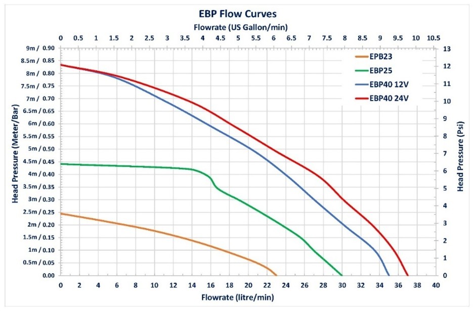
Fig. 3 EBP40 24V PQ curve

It can be expected that y+ > 5 will occur in the CFD simulations at flowrates higher than 10LPM, which is not ideal since 5 < y+ < 30 should be generally avoided for the k-epsilon model due to wall functions not applying well in those y+ values.

Turbulence Model

The model chosen was realizable k-epsilon with enhanced wall treatment. The justification for each part of the chosen model will now be discussed. Firstly, k-epsilon is a robust and well-validated model for turbulent and internal flows. As seen in the y+ calculation, since Re > 2300, we are dealing with turbulent flow. Also, if we were to use k-omega SST, it would lead to increased compute time since y+ < 1 is required to accurately resolve the viscous sublayer. This makes k-epsilon the more attractive choice, especially since we have to do a parametric study with multiple flow rates.

The realizable model was chosen due to its ability to handle strong curvature and strain in the fluid domain. These are the types of characteristics exhibited by water that would be flowing through the motor jacket, especially as temperature increases and viscosity decreases. It also handles pressure gradients at the wall better than the standard k-epsilon model.

Finally, EWT (enhanced wall treatment) was chosen due to its ability to blend viscous sublayer modelling (y+ < 5) and wall functions (y+ > 30) using a blending function for 5 < y+ < 30. In practical terms, it’s good for internal pipe-style flows, which cooling passages are.

The paper linked here validates the selection of our chosen model for internal turbulent pipe flow. The superior model in the paper’s results was determined to be RNG k-epsilon w/ EWT, however in our case the RNG was swapped for realizable due to better performance in complex flows involving recirculation.

All justification for this turbulence model also applies to the CFD done on the cold plates.

Boundary Conditions

A mass flow inlet was used which corresponds to volume flowrates of 5LPM to 30LPM in 5LPM increments:

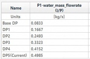
Fig. 4 Parametric design points table in Ansys Fluent

The outlet was a pressure based outlet at 0 gauge pressure. The pressure drop results will be extracted by reporting the mass-weighted average inlet pressure minus the outlet pressure, giving the pressure drop across the motor jacket.

Mesh Sensitivity

All mesh sensitivity runs were conducted at 10LPM. The results can be seen in the table below.

Surface Mesh Min (mm)	Surface Mesh Max (mm)	# of Boundary Layers (-)	First Height of Boundary Layers (mm)	Transition Ratio (-)	Volume Mesh Min (mm)	Volume Mesh Max (mm)	Pressure Drop (Pa)	Pressure Drop Change (%)
0.8	5.12	5	0.01	0.272	0.8	3.2	12,255	-
0.4	2.56	5	0.01	0.272	0.4	1.6	11,913	2.8
0.2	1.28	5	0.01	0.272	0.2	0.8	11,736	1.5
0.1	0.64	5	0.01	0.272	0.1	0.4	11,667	0.6

Table 1 Mesh sensitivity runs for EV6 motor jacket

Ultimately, the finest mesh produced was used in the analysis. In the future, a coarser mesh from the table above should be used to save compute time. This can be done as long as the results change 3% or less to the next mesh size up.

Y+ Contours

Y+ contours for 5LPM and 30LPM are shown below:

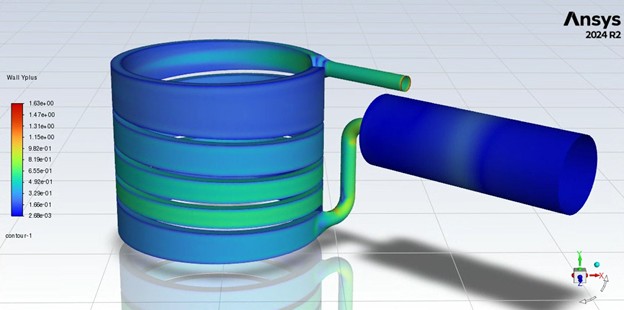
Fig. 5 Y+ contour plot for 5LPM

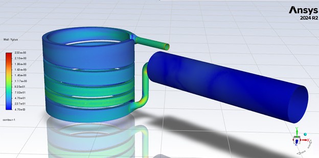
Fig. 6 Y+ contour plot for 30LPM

An enlarged outlet pipe was modelled for the 5LPM run due to issues with the atmospheric pressure outlet causing lots of backflow to achieve the pressure target, resulting in divergence during the simulation. The larger outlet pipe solved these issues and allowed the fluid to recover pressure and exit the fluid domain uniformly.

Note that the 30LPM case initially diverged and required the outlet pipe to be further extended by an additional 3 inches in length in order to converge correctly. The y+ was also re-calculated and the boundary layer height was implemented, as can be seen in the images below.

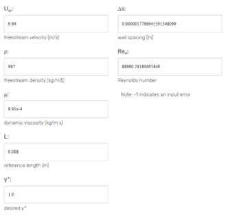
Fig. 7 New y+ calculation and wall spacing used for updated 30LPM case

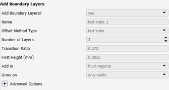
Fig. 8 New boundary layer settings used for updated 30LPM case. Previously, the first height was 0.01mm, and the newly implemented first height given by the y+ calculator was doubled (to 0.0035mm) to overcome excessive solve times. Despite doubling the ideal first wall height, this still resulted in y+ < 5 as seen in the contour plots above

The peak y+ of 1.63 in the 5LPM simulation should be used as a benchmark for future cooling device simulations, since we have the computing power to run this fine of a mesh.

Pressure Drop Results

The pressure drop results for the device can be seen in the table below. The results were taken by outputting the following report from Fluent:

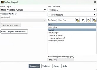
Fig. 9 Reporting pressure drop across a cooling device

Flow (LPM)	Pressure Drop (Pa)
5	3,528
10	11,667
15	21,587
20	25,855
25	47,198
30	63,298

Table 2 Pressure drops for EV6 motor cooling jacket

These pressures will be used to calculate the operating flow and pressure of the cooling system. Mass-weighted average was used over area-weighted average to account for backflow and velocity fluctuations near the inlet and outlet.

Thermal Analysis

Based on previous research conducted during EV4 and EV5, it was determined that the helical design would provide low hydraulic resistance while still achieving adequate thermal conductivity. We decided to stick with this for MACFE 2025, and the thermal results can be seen below.

# of Internal Loops (-)	Inlet Water Temperature (K)	Outlet Water Temperature (K)	Average Wet Area Temperature (K)
4	300	303.9	320.8
5	300	304.2	318.7
6	300	304.9	315.7

Table 3 Thermal analysis for EV6 motor cooling jacket

The motor was modelled as an aluminum volumetric heat source where the heat generated was 3000W. This heat output was determined by establishing a well educated guess for a power request curve from the motors during operation, as we did not have real-world RPM and torque data to work off of.

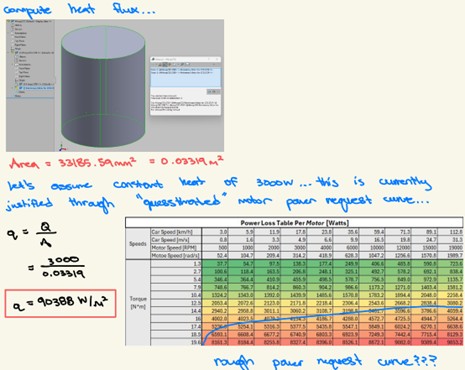
Fig. 10 Computing heat flux based on surface area of the motor and a guesstimated power request curve

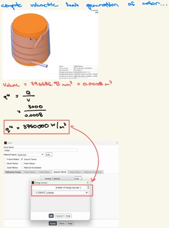
Fig. 11 Computing volumetric heat generation to input as a source term into Ansys Fluent

Ultimately, the 5 loop design was chosen over the 6 loop design even though the 6 loop yielded the lowest average wet area temperature. This is because from the AMK motor datasheet, the maximum coolant increase across the motor surface is 5K, and the 6 loop design would be getting too close to that limit as can be seen in the outlet temperatures reported in Table 3.

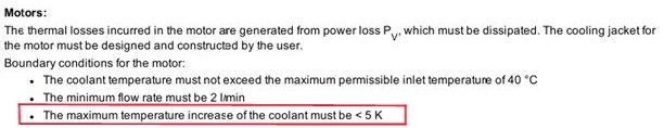
Fig. 12 Maximum temperature increase across AMK motor

---

Cold Plates

The exact same process for the motor jacket analysis was used to determine the hydraulic performance of the cold plates. Note that thermal anaylsis was not done on the cold plates, since the design would be remaining the same as EV5 and therefore we would be relying on the thermal analysis done at that time. Only hydraulic analysis was done to help determine the operating point of the MACFE 2025 cooling loop.

Mesh Sensitivity

All mesh sensitivity runs were conducted at 10LPM. The results can be seen in the table below:

Surface Mesh Min (mm)	Surface Mesh Max (mm)	# of Boundary Layers (-)	First Height of Boundary Layers (mm)	Transition Ratio (-)	Volume Mesh Min (mm)	Volume Mesh Max (mm)	Pressure Drop (Pa)	Pressure Drop Change (%)
0.8	16	7	0.01	0.272	0.8	12.8	2,979	-
0.4	8	7	0.01	0.272	0.4	6.4	2,885	3.2
0.2	4	7	0.01	0.272	0.2	3.2	2,867	0.63
0.1	2	7	0.01	0.272	0.1	1.6	2,864	0.11

Table 4 Mesh sensitivity runs for EV6 cold plate

Ultimately, the finest mesh produced was used in the analysis. In the future, a coarser mesh from the table above should be used to save compute time. This can be done as long as the results change 3% or less to the next mesh size up.

Note that a fifth mesh, coarser than the coarsest one in the current table, was not generated and run due to excessive skewness in the surface mesh. This would have led to completely unrealistic results and was therefore removed from the sensitivity study.

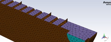
Fig. 13 Surface mesh min 1.6mm, max 32mm. Notice how the pin holes are no longer circular, and the mesh is no longer capturing the model accurately

Y+ Contours

Y+ contours for 5LPM and 30LPM are shown below:

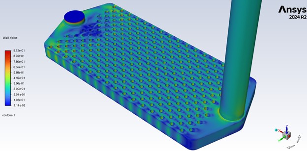
Fig. 14 Y+ contour plot for 5LPM

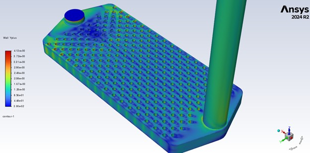
Fig. 15 Y+ contour plot for 30LPM

Although a y+ > 5 was predicted, this did not end up being the case which is a good thing. However, the cause for y+ staying less than 5 at high flowrates should be understood for the future.

An enlarged outlet pipe was modelled due to issues with the atmospheric pressure outlet causing lots of backflow to achieve the pressure target, resulting in divergence during the simulation. The larger outlet pipe solved these issues and allowed the fluid to recover pressure and exit the fluid domain uniformly.

Pressure Drop Results

Flow (LPM)	Pressure Drop (Pa)
5	767
10	2,864
15	6,093
20	10,392
25	15,682
30	22,022

Table 5 Pressure drops for EV6 cold plate

These pressures will be used to calculate the operating flow and pressure of the cooling system.