MACFE 2025 Radiator Selection and Placement
Formula SAE3D CFDAerodynamicsCoolingSoftware DevelopmentThe method to size the EV5 radiator was based on conservative assumptions and hand-calculations. While this was a decent way to justify the radiator size given we did not have an empirical overall HTC, the design and analysis process could benefit from less assumptions as well as a parametric way to calculate the overall HTC for any size of radiator.
The method chosen for this year once again revolves around fundamental heat transfer calculations, however they are combined with the eNTU method to create a robust workflow to solve for hot fluid outlet temperatures. Assumptions are still required for some radiator dimensions (since we can’t measure all of them in-person), however after seeing the outputs in MATLAB it can be said that this method provides a reasonable way for modelling radiators. An overall HTC is also obtained through the MATLAB script, which is then used for the eNTU temperature calculations.
This article also justifies the placement of the MACFE 2025 radiators.
Program Structure
The entire program can be split into 4 main sections as shown in the table below, along with its relevant code. Note that large code snippets which reveal too much of the program are not being shown at this time to allow MAC Formula Electric to maintain a competitive advantage at Formula SAE competitions. Only segments of code which contain textbook heat transfer calculations will be shown in this article.
| Section | Code Snippet |
| Hot fluid (water) calculations | Lines 16-35 |
| Cold fluid (air) calculations | Lines 37-59 |
| eNTU calculations | Lines 61-83 |
| Endurance simulation calculations | Lines 95-156 |
Table 1 The 4 main sections of the radiator sizing calculator. MAC Formula Electric members are encouraged to open the program and identify these sections of code
Before we start breaking down each section, we will talk about the radiator geometry. All of the geometric variables regarding the radiator size were calculated with the help of formulas from this MATLAB tutorial.
This tutorial helped make reasonable calculations for dimensions such as the internal tube dimensions, total surface area of the fins, and the distance between adjacent radiator tubes. The dimensions were provided based on the radiator being analyzed. For example, the EV5 radiator (Yamaha YXR700 Rhino) was measured in-person to obtain the desired dimensions. Other radiators which we wanted to analyze but did not have on hand (e.g. Kawasaki KX450F 2010-2012) were “measured” through online images and reasonable assumptions were made to continue the analysis.
With dimensions established, we can now talk about the hot and cold fluid calculations and why they are being done. The overall goal of these calculations was to be able to calculate a convective HTC for both the fluids, which we could then use to calculate an overall HTC for the radiator being analyzed.
So, in the hot fluid (water) calculations, we can see that we are able to calculate the convective HTC through fundamental heat transfer calculations:
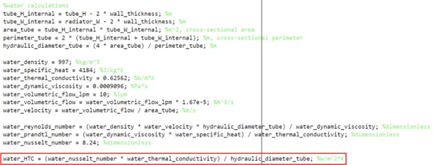
Fig. 1 Convective HTC of water (hot fluid)
Similarly, in the cold fluid (air) calculations, we obtain a convective HTC:
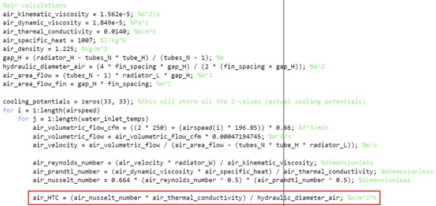
Fig. 2 Convective HTC of air (cold fluid)
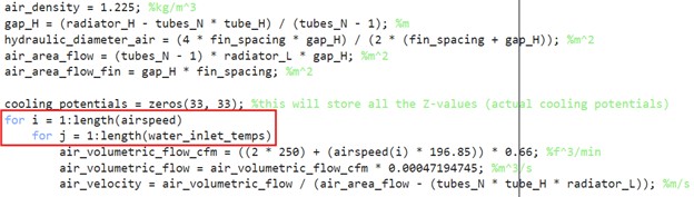
Fig. 3 Air HTC calculated over arrays of speed (0 to 32m/s) and inlet water temps (28 to 60degC)
In Figure 3, the air and overall HTCs are iteratively calculated over arrays of airspeed and inlet water temps. This was done to quantify a given radiator’s performance in a “performance map” through the implementation of the eNTU method. This shows the cooling potential of the radiator with respect to air speed and water inlet temperature, as seen below:
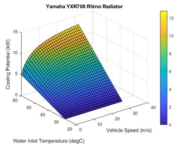
Fig. 4 Radiator “performance map” of Yamaha YXR700 Rhino radiator, which was the radiator used for EV3, EV4, and EV5
The performance map is a good starting point to understand the theoretical cooling capabilities of given radiators, however it does not tell the full story of how water temperatures change over a given amount of driving time. Ultimately, this is what we need to know to ensure the water temperatures do not exceed the limits provided in the AMK motor and inverter datasheets.
To plot water temperature over time, we start with an initial water temperature of 27degC. We then run the code for a simulated driving cycle of 30 minutes. The heat loads and vehicle speeds for the duration of 30 minutes are obtained from an OptimumLap endurance simulation around Michigan’s FSAE track, which was given by the Powertrain subteam. This means that at every timestep, we calculate the water temperature for the given heat load and radiator cooling potential, and plot the water temperature over time once the simulation has finished.
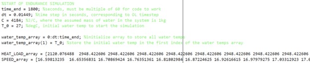
Fig. 5 Initial code to start the simulation. HEAT_LOAD_array and SPEED_array are extracted values from OptimumLap. Each value in both of the arrays corresponds to one time step of 0.01449 seconds (which is the frequency OptimumLap ran its simulation at)
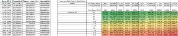
Fig. 6 Heat load map (coloured chart on the right) from OptimumLap with respect to motor speed and motor torque. The results in the map are then assigned to each incremental speed and torque value (on the left) to create an array of heat loads, which are finally fed into HEAT_LOAD_array in MATLAB. Special thank you to Owen Spira for helping create the Excel map
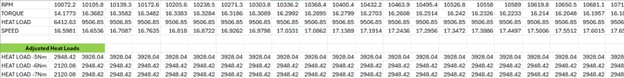
Fig. 7 Simulations were also conducted at adjusted heat loads with reduced torques, since the motors can’t sustain 21Nm of torque continuously. So, to plot more realistic results, 5-7Nm of torque were taken away from the results to re-run the simulation and drop the heat loads, ultimately reducing the outlet water temperature
The final plots looked like the ones shown below. All radiators were simulated, and the best one was chosen based on its performance map and endurance simulation results.
Fig. 8 Yamaha YXR700 Rhino radiator
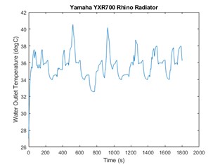
Fig. 9 Yamaha YXR700 Rhino radiator, torque values reduced by 7Nm at each time step. This is a more realistic result, since the motors can only do 13.8Nm continuously
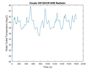
Fig. 10 Honda CR125/125R radiator, torque values reduced by 7Nm at each time step
Final Radiator and Fan Selection
In the end, we ended up choosing the Honda CR125/125R radiator, as the radiator kept the outlet temperature of the water at or below 45degC. Although the water must be 30degC at the inverter and 40degC at the inlet of the motors (from the datasheet), this is highly difficult to achieve as the ambient temperatures at Michigan International Speedway reach 27degC alone. This means the inverter will have to de-rate to prevent overheating no matter which radiator was chosen, and this issue has been addressed to the Electrical and Software and Vehicle Controls subteams to be implemented.
The radiator also provides a good drop in physical size which was the entire goal of this project, as shown in the table below.
| Radiator | Length (in) | Width (in) | Height (in) | Reference |
| Yamaha YXR700 Rhino | 18.66 | 12.87 | 3.35 | https://www.mishimoto.com/yamaha-yxr700-rhino-aluminum-radiator-08-11.html |
| Honda CR125/125R Radiator | 11.40 | 6.20 | 1.80 | https://49ccscoot.proboards.com/thread/21059/radiator-dimensions-info-thread |
Table 2 Yamaha YXR700 Rhino vs. Honda CR125/125R radiator
Due to budget constraints regarding import/shipping fees, as well as mounting/assembly considerations, we ended up purchasing the Kimpex 164610 radiator as it is meant to be used on a slightly higher power-output motorbike compared to the Honda CR125/125R. Due to this fact and their similar reported sizes, we were confident about its cooling performance and purchased the radiator. References for each radiator are in the table below.
| Radiator | Reference |
| Honda CR125/125R Radiator | https://49ccscoot.proboards.com/thread/21059/radiator-dimensions-info-thread |
| Kimpex 164610 | https://fortnine.ca/en/kimpex-replacement-radiator-164610 |
Table 3 Honda CR125/125R radiator and Kimpex 164610 references
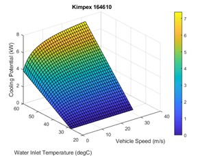
Upon receiving the new radiators, they were measured and re-run through the MATLAB code to get a final performance map and endurance simulation. The results can be seen below.
 |
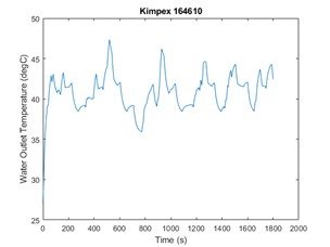 |
Figs. 11 and 12 Kimpex 164610 performance map and endurance simulation
Although the results are slightly worse than the initially chosen Honda CR125/125R radiator, it should be noted that general radiator performance is expected to be better than the MATLAB simulation as real-life torque requests will not be as instantaneous as a simulation (i.e. the driver will slowly apply the throttle, not instantly). This data would help reduce the heat load per time step, ultimately reducing outlet water temperatures.
The fans chosen were the Delta FFB1424UHE-M fans, as they offer increased static pressure and volumetric flow over our old fans. The chosen setup was 2 fans per radiator (for a total of 4 fans), however due to budget constraints we had to stick with our old fans. A comparison between the 2 fan models can be seen in the table below for future reference.
| Fan | Max. Flow (CFM) | Max. Pressure (mmH20) | Reference |
| Delta FFB1424VHG-EP (old) | 252.11 | 16.36 | https://www.delta-fan.com/products/ffb1424vhg-ep.html |
| Delta FFB1424UHE-M (new, recommended) | 367.62 | 41.75 | https://www.delta-fan.com/products/ffb1424uhe-m.html |
Table 4 Old vs. new recommended Delta fans
Radiator Placement
During the 2024 Formula SAE Electric competition, David Caples pointed out a worrying conclusion of rear-mounted radiators. Although rear-mounted setups are very attractive due to less drag and neater packaging, the total pressure behind the car drops drastically as speed increases, ultimately meaning there is less air mass to physically move through the radiator. Since we hadn’t tested if the fans could extract the total pressure from underneath the car and move it through the radiator, this raised doubts about the theoretical cooling performance.

Fig. 13 MAC EV5 rear-mounted radiator setup with 2 fans
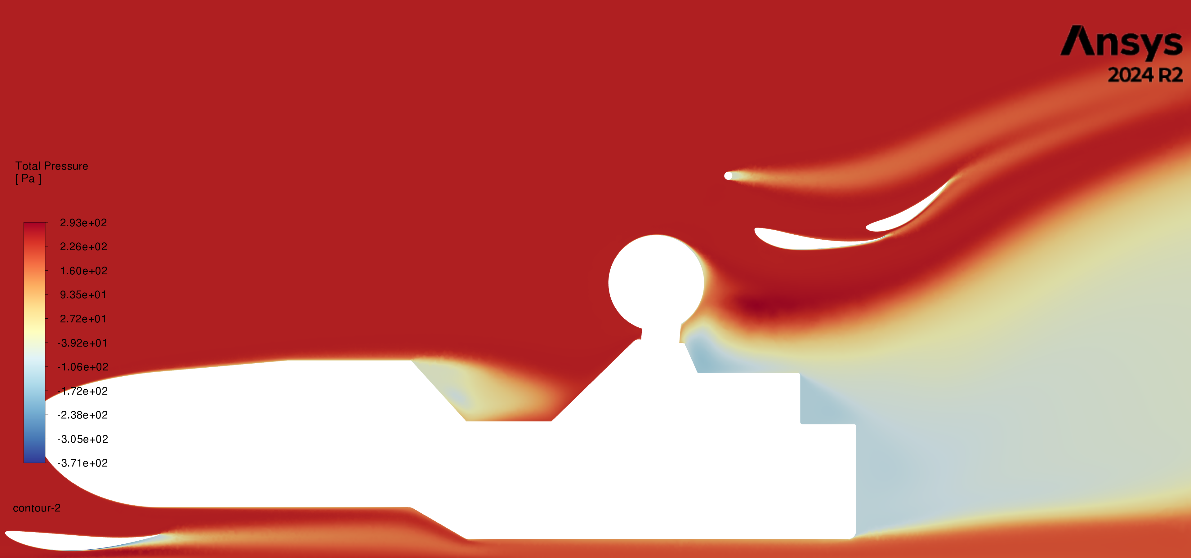
Fig. 14 Total pressure plot of centerline of MACFE 2025 at 20m/s. Note the total pressure conserved underneath the chassis, and the large low-pressure zone behind the vehicle
If a test bench is made with an obstruction to mimic the chassis and a rear-mounted radiator, and an anemometer is used to measure exit mass airflow and chassis-floor mass airflow, and the exit flow is within a reasonable percentage of chassis-floor flow, it could be feasible to have rear-mounted radiators again (or radiators mounted behind the rear suspension arms). This test would help us be confident in a rear-mounted radiator design which is not overly-starved of mass airflow.
For MACFE 2025, we decided to play it safe and mount the radiators in a traditional sidepod area, due to our confidence in there being high total pressure to feed the radiators and get as close to the designed cooling performance as possible. The total pressure plot below highlights this.
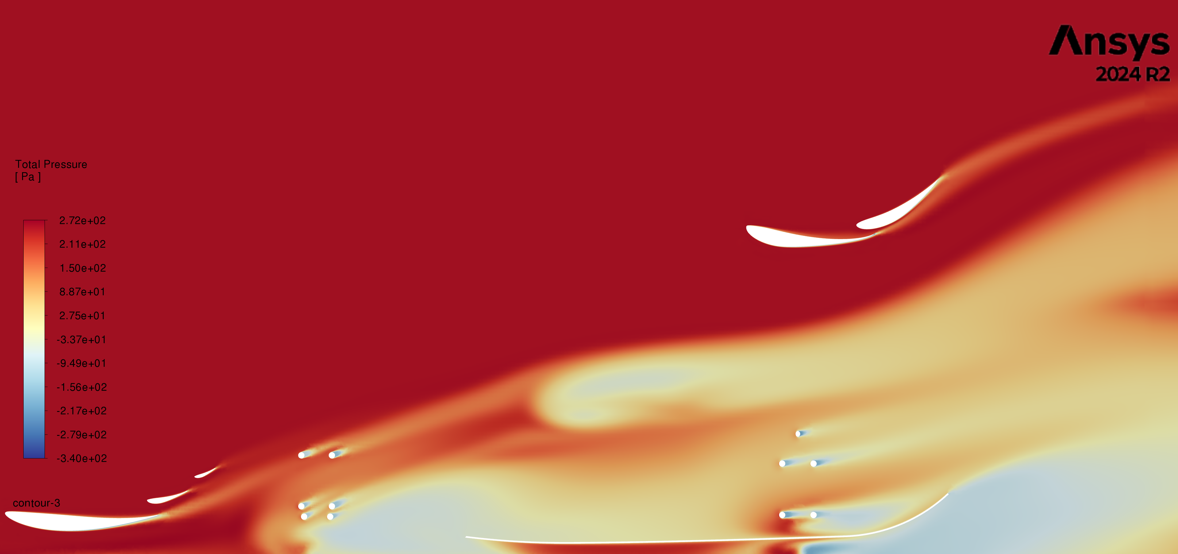
Fig. 15 Total pressure plot of MACFE 2025 at 20m/s. Cut plane is the midplane between inboard rear tire and chassis wall
The radiators were mounted fore of the rear suspension arms to place them in the highest total pressure airflow.

Fig. 16 Side-mounted radiators on MACFE 2025
References
| Reference | Context |
| https://www.mathworks.com/help/hydro/ug/modeling-heat-exchangers.html | Basic radiator modelling |
| https://www.filipjander.com/2020/09/designing-formula-sae-cooling-system.html | Inspiration for analytical radiator model |
| https://www.sciencedirect.com/science/article/abs/pii/S2214785322074302 | Inspiration for analytical radiator model |
| https://www.engineersedge.com/heat_transfer/nusselt_number_13856.htm | Nusselt numbers used in MATLAB code |
| https://www.engineersedge.com/calculators/thermal_conductivities_liquids_and_gases_16304.htm | Thermal conductivities used in MATLAB code |
| https://www.engineersedge.com/physics/viscosity_of_air_dynamic_and_kinematic_14483.htm | Air properties used in MATLAB code |
| https://www.grc.nasa.gov/www/k-12/airplane/heat.html | Fundamental heat transfer |
| https://www.mheducation.com/highered/product/Heat-and-Mass-Transfer-Fundamentals-and-Applications-Cengel.html | Fundamental heat transfer (eNTU calculations) |
Table 5 Additional references for analytical model development